|
VII. EXAMPLE OF TIME-DOMAIN SIGNAL PROCESSING AND ANALYSIS We will analyze in some detail a commercial portable clock, Serial No. 102. This cesium was measured against another commercial cesium whose stability was well-documented and verified to be better than the one under test. Plotted in figure 7.1 are the residual time deviations after removing a mean frequency of 4.01 parts in 1013. Applying the methods described in section IV and section V, we generated the s y(t ) diagram shown in figure 7.2. One observes that the last two points are proportional to t +1 and one is suspicious of a significant frequency drift. If one calculates the drift knowing that s y(t ) is equal to the drift times t /%2 a drift of 1.22 x 10⁻¹⁴ per day is obtained. A linear least squares to the frequency was removed and sections IV and V were applied again. The linear least squares fit showed a drift of 1.23 x 10⁻¹⁴ per day, which is in excellent agreement with the previous calculated value obtained from s y(t ). typically, the linear least squares will give a much better estimate of the linear frequency drift than will the estimate from s y(t ) being proportional to t +1. Figure 7.3 gives the plot of the time residuals after removing the linear least squares and figure 7.4 is the corresponding s y(t ) vs. t diagram. From the 33 days of data, we have used the 90% confidence interval to bracket the stability estimates and one sees a reasonable fit corresponding to white noise frequency modulation at a level of 4.4 x 10⁻¹¹ t -2. This seemed excessive in terms of the typical performance of this particular cesium and in as much as we were doing some other testing within the environment, such as working on power supplies and charging and discharging batteries, we did some later tests. Figure 7.5 is a plot of s y(t ) after the standard had been left alone in a quiet environment and had been allowed to age for about a week. One observes that the white noise frequency modulation level is more than a factor of 4 improved over the previous data. This led us to do some studies on the effects of the power supply on the cesium frequency as one is charging and discharging batteries, which proved to be significant. One notices in figure 7.4 that the s y(t ) values plotted are consistent within the error bars with flicker noise frequency modulation. This is more typical of the kind of noise one would expect due to such environmental perturbations as discussed above. 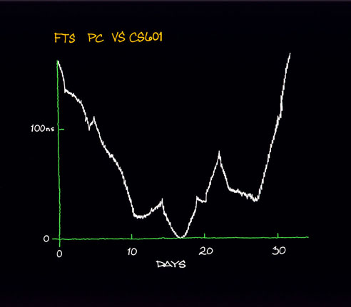 Figure 7.1 Careful time- and/or frequency-domain analyses can lead to significant insights into problems and their solutions and is highly recommended by the authors. The frequency-domain techniques will be next approached. 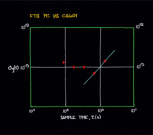 Figure 7.2 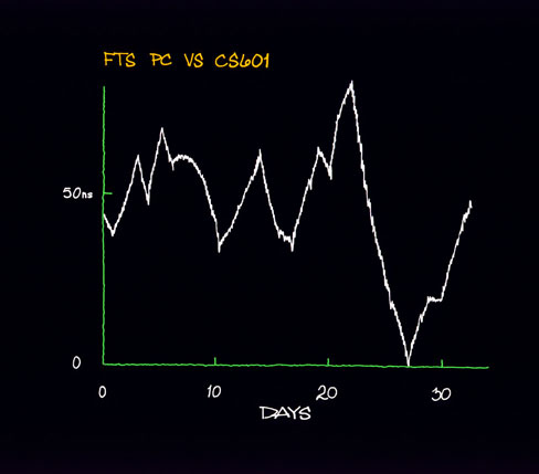 Figure 7.3 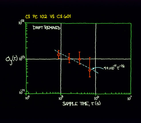 Figure 7.4 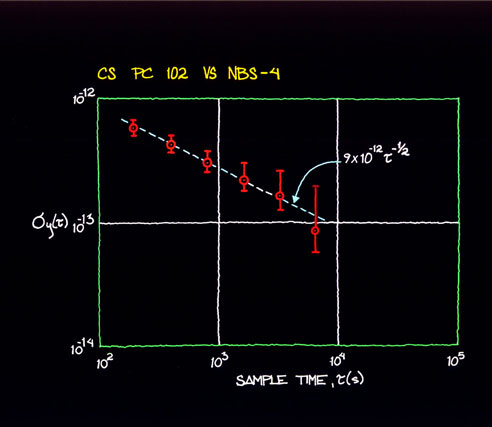 Figure 7.5
Main Page |
