|
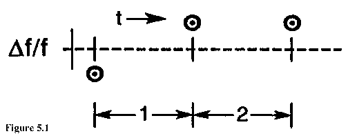
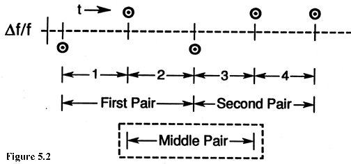
V. CONFIDENCE OF THE ESTIMATE AND OVERLAPPING SAMPLES One can imagine taking three phase or time measurements of one oscillator relative to another at equally spaced intervals of time. From this phase data one can obtain two, adjacent values of average frequency. From these two frequency measurements, one can calculate a single Allan (or two-sample) variance (see fig. 5.1). Of course this variance does not have high precision or confidence since it is based on only one frequency difference. Statisticians have considered this problem of quantifying the variability of quantities like the two-sample variance. Conceptually, one could imagine repeating the above experiment many times (of taking the three phase points and calculating the variance) and even calculating the distribution of the values.  For the above cited experiment we know that the results are distributed like the statistician's chi-square distribution with one degree of freedom. That is, we know that for most common oscillators the first difference of the frequency is a normally distributed variable with the typical bell-shaped curve and zero mean. However, the square of a normally distributed variable is NOT normally distributed. That is easy to see since the square is always positive and the normal curve is completely symmetric and negative values are as likely as positive. The resulting distribution is called a chi-square distribution, and it has ONE "degree of freedom" since the distribution was obtained by considering the squares of individual (i.e., one independent sample), normally distributed variables. In contrast, if we took five phase values, then we could calculate four consecutive frequency values, as in figure 5.2. We could then take the first pair and calculate a variance, and we could calculate a second variance from the second pair (i.e., the third and fourth frequency measurements). The average of these two variances provides an improved estimate of the "true" variance, and we would expect it to have a tighter confidence interval than in the previous example. This could be expressed with the aid of the chi-square distribution with TWO degrees of freedom. However, there is another option. We could also consider the two-sample variance obtained from the second and third frequency measurements. That is the middle sample variance. Now, however, we're in trouble because clearly this last variance is NOT independent
 of the other two. Indeed, it is made up of parts of each of the other two. This does NOT mean that we can't use it for improving our estimate of the "true" variance, but it does mean that we can't just assume that the new average of three variances is distributed as chi-square with three degrees of freedom. Indeed, we will encounter chi-square distributions with fractional degrees of freedom. And as one might expect, the number of degrees of freedom will depend upon the underlying noise type, that is, white FM, flicker FM, or whatever. Before going on with this, it is of value to review some concepts of the chi-square distribution. Sample variances (like sample Allan Variances) are distributed according to the equation:
where S2 is the sample Allan Variance, X2 is chi-square, d.f. is the number of degrees of freedom (possibly not an integer), and s 2 is the "true" Allan Variance we're all interested in knowing--but can only estimate imperfectly. Chi-square is a random variable and its distribution has been studied extensively. For some reason, chi-square is defined so that d.f., the number of degrees of freedom appears explicitly in eq (5.1). Still, X2 is a (implicit) function of d.f., also. The probability density for the chi-square distribution is given by the relation
 is the gamma function, defined by the integral
Chi-square distributions are useful in determining specified confidence intervals for variances and standard deviations. Here is an example. Suppose we have a sample variance s2 = 3.0 and we know that this variance has 10 degrees of freedom. (Just how we can know the degrees of freedom will be discussed shortly.) Suppose also that we want to know a range around our sample value of s2 = 3.0 which "probably" contains the true value, s 2. The desired confidence is, say, 90%. That is, 10% of the time the true value will actually fall outside of the stated bounds. The usual way to proceed is to allocate 5% to the low end and 5% to the high end for errors, leaving our 90% in the middle. This is arbitrary and a specific problem might dictate a different allocation. We now resort to tables of the chi-square distribution and find that for 10 degrees of freedom the 5% and 95% points correspond to: C 2(.05) = 3.94 for d.f. = 10 (5.4) C 2(.95) = 18.3 (5.5) Thus, with 90% probability the calculated sample variance, s2, satisfies the inequality:
or, taking square roots: 1.28 £ s £ 2.76 (5.7) Now someone might object to the form of eq (5.7) since it seems to be saying that the true sigma falls within two limits with 90% probability. Of course, this is either true or not and is not subject to a probabilistic interpretation. Actually eq (5.7) is based on the idea that the true sigma is not known and we estimate it with the square root of a sample variance, s2. This sample variance is a random variable and is properly the subject of probability, and its value (which happened to be 3.0 in the example) will conform to eq (5.7) nine times out of ten. Typically, the sample variance is calculated from a data sample using the relation:
where it is implicitly assumed that the xn's are random and uncorrelated (i.e., white)
and where Thus, for the case of white xn, and a conventional sample variance (i.e., eq (5.8)), the number of degrees of freedom are given by the equation: d.f. = N-1 (5.9) The problem of interest here is to obtain the corresponding equations for Allan Variances using overlapping estimates on various types of noise (i.e., white FM, flicker FM, etc.). Other authors (Lesage and Audoin, and Yoshimura) have considered the question of the variance of the Allan Variances without regard to the distributions. This is, of course, a closely related problem and use will be made of their results. These authors considered a more restrictive set of overlapping estimates than will be considered here, however.
Main Page |


 is the sample mean calculated from the
same data set. If all of this is true, then
s2 is chi-square distributed and has N-1 degrees
of freedom.