|
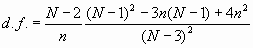
VI. MAXIMAL USE OF THE DATA AND DETERMINATION OF THE DEGREES OF FREEDOM. 6.1 Use of Data Consider the case of two oscillators being compared in phase and exactly N values of the phase difference are obtained. Assume that the data are taken at equally spaced intervals, t 0. From these N phase values, one can obtain N-1 consecutive values of average frequency and from these one can compute N-2 individual, sample Allan Variances (not all independent) for t = t 0. These N-2 values can be averaged to obtain an estimate of the Allan Variance at t = t 0. The variance of this variance has been calculated by the above cited authors. Using the same set of data, it is also possible to estimate the Allan Variances for integer multiples of the base sampling interval, t = nt 0. Now the possibilities for overlapping sample Allan Variances are even greater. For a phase data set of N points one can obtain exactly N-2n sample Allan Variances for t = nt 0. Of course only a fraction of these are generally independent. Still the use of ALL of the data is well justified (see fig. 6.1). 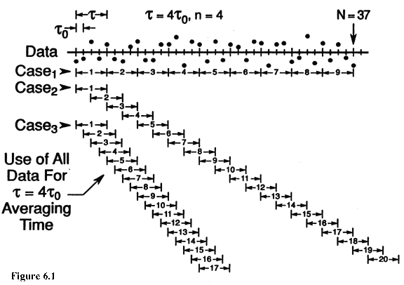 Consider the case of an experiment extending for several weeks in duration with the aim of getting estimates of the Allan Variance for tau values equal to a week or more. As always the purpose is to estimate reliably the "true" Allan Variance as well as possible--that is, with as low an uncertainty as possible. Thus one wants to use the data as efficiently as possible since obtaining more data can be very expensive. The most efficient procedure is to average all possible sample Allan Variances of a given tau value that one can compute from the data. The problem comes in estimating how tight the confidence intervals really are--that is, in estimating the number of degrees of freedom. Clearly, if one estimates the confidence intervals pessimistically, then more data is needed to reach a specified tolerance, and that can be expensive. The other error of over-confidence in a questionable value can be even more expensive. Ideally one has realistic confidence estimates for the most efficient use of the data, which is the intent of this writing. 6.2 Determining the Degrees of Freedom In principle, it should be possible to determine analytically the equations corresponding to eq (5.9) for all cases of interest. Unfortunately the analysis becomes quite complicated. Exact computer algorithms were devised for the cases of white phase noise, white frequency modulation and random walk FM. For the two flicker cases (i.e., flicker FM and PM) a completely empirical approach was used. Due to the complexity of the computer programs, empirical fits were devised for all five noise types. The approach used is based on three equations relating to the chi-square distribution:
where the expression E[ C 2] means the "expectation," or average value of C , Var[C 2] is the variance of C 2, and d.f. is the number of degrees of freedom. A computer was used to simulate phase data sets of some length, N, and then Allan Variances with t = nt 0 were calculated for all possible samples. This "experiment" was repeated at least 1000 times using new simulated data sets of the same spectral type, and always of the same length, N. Since the data were simulated on a computer, the "true" Allan Variance, s 2, was known for many of the noise models and could be substituted into eq (6.1). From the 1000 values of s2/s 2, distributions and sample variances were obtained. The "experimental" distributions were compared with theoretical distributions to verify that the observed distributions truely conformed to the chi-square distribution. The actual calculation of the degrees of freedom were made using the relation:
which can be deduced from eqs (6.1), (6.2), and (6.3). The Var(s2) was estimated by the sample variance of the 1000 values of the average Allan Variances, each obtained from a phase data set of length N. Of course this had to be repeated for various values of N and n, as well as for each of the five common noise types: white PM, flicker PM, white FM, flicker FM, and random walk FM. Fortunately, certain limiting values are known and these can be used as checks on the method. For example, when (N-1)/2=n, only one Allan Variance is obtained from each data set and one should get about one degree of freedom for eq (6.3), which was observed in fact. Also for n=1 the "experimental" conditions correspond to those used by Lesage and Audoin, and by Yoshimura. Indeed, the method also was tested by verifying that it gave results consistent with eq (5.9) when applied to the conventional sample variance. Thus, combining eq (6.4) with the equations for the variance of the Allan Variances from Lesage and Audoin and Yoshimura, one obtains:
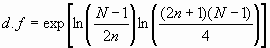
for n=1. Unfortunately, their results are not totally consistent with each other and for that reason the Flicker PM case is not included. Where other inconsistencies arose the value in best agreement with the "experimental" results was chosen. The empirical equations which were fit to the "experimental" data and the known values are summarized below:
The figures in Appendix I demonstrate the fit to the "experimental" data. It is appropriate to give some estimate of just how well these empirical equations approach the "true" values. The equations have approximately (a few percent) the correct asymptotic behavior at n=1 and n=(N-1)/2. In between, the values were tested (using the simulation results) over the range of N=5 to N=1025 for n=1 to n=(N-2)/2 changing by octaves. In general, the fit was good to within a few percent. We must acknowledge that distributional problems with the random number generators can cause problems, although there were several known values which should have revealed these problems if they are present. Also for three of the noise types the exact number of degrees of freedom were calculated for many values of N and n and compared with the "Monte Carlo" calculations. The results were all very good. Appendix I presents the data in graphical form. All values are thought to be accurate to within one percent or better for the cases of white PM, white FM, and random walk FM. A larger tolerance should be allowed for the flicker cases.
Main Page |


![df=[3(N-1)/2n-2(N-2)/N]=4n^2/(4n^2+5)](Properties_images/Image52.gif)