XI. TRANSLATION FROM FREQUENCY DOMAIN STABILITY MEASUREMENT TO TIME DOMAIN STABILITY MEASUREMENT AND VICE-VERSA.
11.1 Procedure
Knowing how to measure Sf (f) or Sy(f) for a pair of oscillators, let us see how to translate the power-law noise process to a plot of s y2(t ), the two-sample variance. First, convert the spectrum data to Sy(f), the spectral density of frequency fluctuations (see sections III and VIII). There are two quantities which completely specify Sy(f) for a particular power-law noise process: (1) the slope on a log-log plot for a given range of f and (2) the amplitude. The slope we shall denote by "a "; therefore fa is the straight line (on log-log scale) which relates Sy(f) to f. The amplitude will be denoted "ha "; it is simply the coefficient of f for a range of f. When we examine a plot of spectral density of frequency fluctuations, we are looking at a representation of the addition of all the power-law processes (see sec. IX). We have
 | (11.1) |
In section IX, five power-law noise processes were outlined with respect to Sf (f). These five are the common ones encountered with precision oscillators. Equation (8.7) relates these noise processes to Sy(f). One obtains
| with respect to Sy(f) | slope on log-log paper |
| 1. Random Walk FM | (f-2)...................................a = -2 |
| 2. Flicker FM | (f-1)...................................a = -1 |
| 3. White FM | (1)....................................a = 0 |
| 4. Flicker fM | (f).....................................a= 1 |
| 5. White fM | (f2)....................................a = 2 |
Table 11.1 is a list of coefficients for translation from s y2(t ) to Sy(f) and from Sf (f) to s y2(t ). In the table, the left column is the designator for the power-law process. Using the middle column, we can solve for the value of Sy(f) by computing the coefficient "a" and using the measured time domain data s y2(t ). The rightmost column yields a solution for s y2(t ) given frequency domain data Sf (f) and a calculation of the appropriate "b" coefficient.
TABLE 11.1
|
|
|
|
|
2 (white phase) |
|
|
|
1 (flicker phase) |
|
|
|
0 (white frequency) |
2t |
|
|
-1 (flicker frequency) |
|
|
|
-2 (random walk frequency) |
|
|


Conversion table from time domain to frequency domain and from frequency domain to time domain for common kinds of interger power law spectral densities; fb(= w h/2p ) is the measurement system bandwidth. Measurement response should be within 3 dB from D.C. to fh (3 dB down high-frequency cutoff is at fh).
EXAMPLE
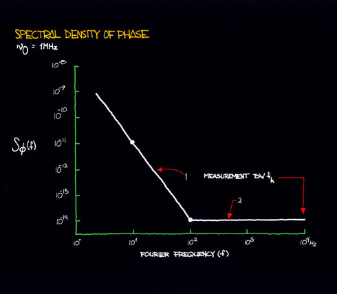
Figure 11.1
:
In the phase spectral density plot of figure 11.1, there are two power-law noise processes for oscillators being compared at 1 MHz. For region 1, we see that when f increases by one decade (that is, from 10 Hz to 100 Hz), Sf (f) goes down by three decades (that is, from 10-11 to 10-14). Thus, Sf (f) goes as 1/f3 = f-3. For region 1, we identify this noise process as flicker FM. The rightmost column of table 11.1 relates s 2y(t ) to Sf (f). The row designating flicker frequency noise yields:
 | (11.2) |
One can pick (arbitrarily) a convenient Fourier frequency f and determine the corresponding values of Sf (f) given by the plot of figure 11.1. Say, f = 10, thus Sf (10) = 10-11. Solving for s 2y(t ), given à0 = 1 MHz, we obtain:
 | (11.3) |
therefore, s y(t ) = 1.18 ´ 10-10. For region 2, we have white PM. The relationship between s 2y(t ) and Sf (f) for white PM is:
 | (11.4) |
Again, we choose a Fourier frequency, say f = 100, and see that Sf (100) =
10-14. Assuming fh = 104 Hz, we thus obtain:
 | (11.5) |
therefore
 | (11.6) |
The resultant time domain characterization is shown in figure 11.2.
Figure 11.2
Figures 11.3 and 11.4 show plots of time-domain
stability and a translation to frequency
domain. Since table 11.1 has the coefficients
which connect both the frequency and time
domains, it may be used for translation to
and from either domain.
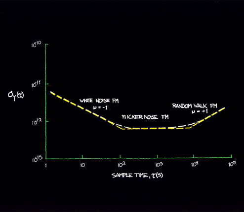
Figure 11.3
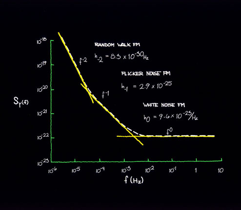
Figure 11.4
Main Page Table of Contents
Go to section:
Summary and Introduction
I
II
III
IV
V
VI
VII
VIII
IX
X
XI
XII
Conclusion
References