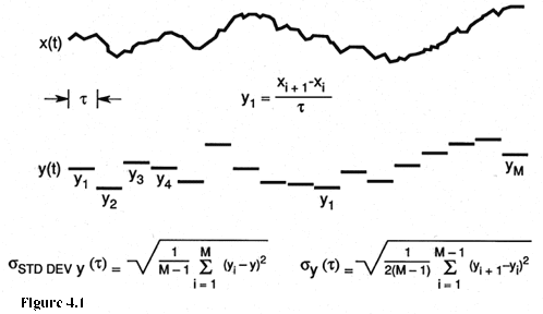
IV. ANALYSIS OF TIME DOMAIN DATA

Suppose now that one is given the time or frequency fluctuations between a pair of precision oscillators measured, for example, by one of the techniques outlined in section I, and a stability analysis is desired. Let this comparison be depicted by figure 4.1. The minimum sample time is determined by the measurement system. If the time difference or the time fluctuations are available then the frequency or the fractional frequency fluctuations may be calculated from one period of sampling to the next over the data length as indicated in figure 4.1. Suppose further there are M values of the fractional frequency y_i. Now there are many ways to analyze these data. Historically, people have typically used the standard deviation equation shown in figure 4.1, s _{std. dev.}(t ), where y is the average fractional frequency over the data set and is subtracted from each value of y_i before squaring, summing and dividing by the number of values minus one, (M-1), and taking the square root to get the standard deviation. At NBS (now NIST), we studied what happens to the standard deviation when the data set may be characterized by power law spectra which are more dispersive than classical white noise frequency fluctuations. In other words, if the fluctuations are characterized by flicker noise or any other non-white-noise frequency deviations, what happens to the standard deviation for that data set? One can show that the standard deviation is a function of the number of data points in the set; it is also a function of the dead time and of the measurement system bandwidth. For example, using flicker noise frequency modulation as a model, as the number of data points increases, the standard deviation monotonically increases without limit. Some statistical measures have been developed which do not depend upon the data length and which are readily usable for characterizing the random fluctuations in precision oscillators. The IEEE has adopted a standard measure known as the "Allan variance" taken from the set of useful variances developed, and an experimental estimation of the square root of the Allan variance is shown as the bottom right equation in figure 4.1. This equation is very easy to implement experimentally as one simply need add up the squares of the differences between adjacent values of y_i, divide by the number of them and by two, and take the square root. One then has the quantity which the IEEE subcommittee has recommended for specification of stability in the time domain--denoted by s _y(t ).

Figure 4.1 is a simulated plot of the time fluctuations, x(t) between a pair of oscillators and of the corresponding fractional frequencies calculated from the time fluctuations each averaged over a sample time t . At the bottom are the equations for the standard deviation (left) and for the time-domain measure of frequency stability as recommended by the IEEE (right).

where the brackets "<>" denote infinite time average. In practice this is easily estimated from a finite data set as follows:

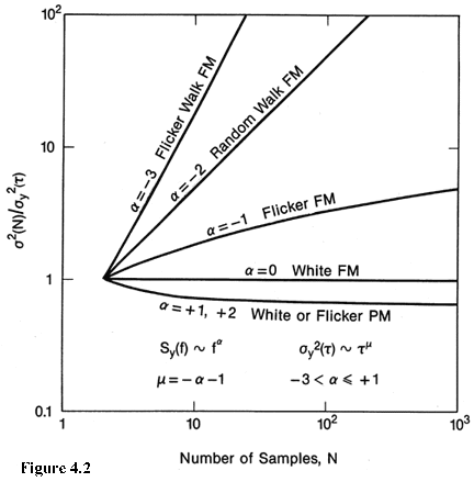
where the y_i are the discrete frequency averages as illustrated in figure 4.1.

 One would like to know how s _y(t ) varies with the sample time, t . A simple trick that one can use that is very useful, if there is no dead time, is to average the values for y₁ and y₂ and call that a new y₁ averaged over 2t , similarly average the values for y₃ and y₄ and call that a new y₂ averaged over 2t etc., and finally apply the same equation as before to get s _y(2t ). One can repeat this process for other desired integer multiples, m, of t , and from the same data set generate values for s _y(mt ) as a function of mt from which one may be able to infer a model for the process that is characteristic of this pair of oscillators. If one has dead time in the measurements adjacent pairs cannot be averaged in an unambiguous way to simply increase the sample time. One has to retake the data for each new sample time--often a very time consuming task. This is another instance where dead time can be a problem.

How the classical variance (standard deviation squared) depends on the number of samples is shown in figure 4.2. Plotted is the ratio of the standard deviation squared for N samples to the standard deviation squared for 2 samples, < s ²(2,t )>, which is the same as the Allan variance, s _y²(t ). One can see the dependence of this standard deviation upon the number of samples for various kinds of power law spectral densities commonly encountered as reasonable models for many important precision oscillators. Note, s _y²(t ) has the same value as the classical variance for the classical noise case (white noise FM). One main point of figure 4.2 is simply to show that with the increasing data length the standard deviation of the common classical variance is not well behaved for the kinds of noise processes that are very often encountered in most of the precision oscillators of interest.

Figure 4.2: The ratio of the time average of the standard deviation squared for N samples over the time average of a two sample standard deviation squared as a function of the number of samples, N. The ratio is plotted for various power law spectral densities that commonly occur in precision oscillators.

The figure illustrates one reason why the standard deviation is not a convenient measure of frequency stability; i.e., it may be very important to specify how many data points are in a data set if you use the standard deviation.

One may combine eq (1.4) and eq (4.1), which yields an equation for s _y(t ) in terms of the time difference or time deviation measurements.

which for N discrete time readings may be estimated as,

where the i denotes the number of the reading in the set of N and the nominal spacing between readings is t . If there is no dead time in the data and the original data were taken with a sample time t ₀, a set of x_i's can be obtained by integrating the y_i's

(4.5)

Once we have the x_i's, we can pick t in eq (4.4) to be any integer multiple of t ₀, i.e., t = mt ₀:

(4.6)